Chapter 1: Introduction to Program Evaluation
Epigraphs
“Not everything that can be counted counts, and not everything that counts can be counted.” — William Bruce Cameron, Informal Sociology (1963)
“Evaluation is the systematic application of social research procedures for assessing the conceptualization, design, implementation, and utility of social intervention programs.” — Peter H. Rossi, Mark W. Lipsey, and Gary T. Henry, Evaluation: A Systematic Approach (paraphrasing their working definition)
Opening Case: Did the National Supported Work Demonstration Raise Earnings?
In the mid-1970s, the Manpower Demonstration Research Corporation ran the National Supported Work (NSW) Demonstration — a job-training program that gave disadvantaged workers (long-term welfare recipients, ex-offenders, former drug users, school dropouts) up to a year of subsidized, gradually more demanding work experience, on the theory that it would build the skills and habits that lead to real, unsubsidized employment. The intended outcome was concrete and dollar-denominated: higher earnings after the program ended.
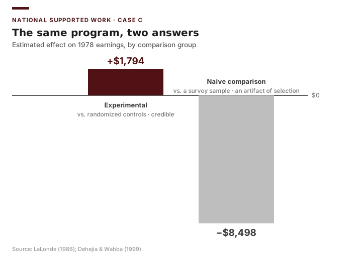
What made NSW unusual is that it was run as a randomized experiment. Eligible applicants were assigned by chance either to the program (treatment) or to a control group that did not get the subsidized jobs. Among the treated men, 1978 earnings averaged $6,349 (n = 185); among the controls, $4,555 (n = 260). The difference — +$1,794 — is a credible estimate of what the program actually caused, because randomization made the two groups comparable on everything except the program itself.
Here is the part that should unsettle every manager. Suppose NSW had not been run as an experiment. Suppose, as is far more common, an analyst had simply compared the treated workers to a large group of similar-looking people drawn from a national survey (the Current Population Survey, n ≈ 16,000) who did not enter the program. That naive observational comparison yields −$8,498 — the program appears to lower earnings by more than eight thousand dollars. The sign flips. A real, effective program looks harmful, purely because the comparison group was the wrong one. Robert LaLonde (1986) used exactly this contrast to put a generation of nonexperimental evaluations on trial, and Dehejia and Wahba (1999) made the NSW data the most-studied teaching case in all of program evaluation.
The gap between +$1,794 and −$8,498 is not a rounding error or a modeling quibble. It is the difference between an honest counterfactual and a misleading one — and it is the situation public managers face constantly: a program exists, money is at stake, decisions loom, and the available evidence describes activity, or the wrong comparison, rather than effect.
Guiding Questions
- What is the difference between what a program did and what difference the program made?
- How can the same program look beneficial under one comparison and harmful under another?
- How is evaluation different from the monitoring reports a manager already produces?
Why This Chapter Matters
Public and nonprofit managers are accountable for results, not just effort. Legislatures, councils, boards, and funders increasingly ask programs to show evidence of effectiveness, and “we served a lot of people” is no longer a sufficient answer. Program evaluation is the craft of producing credible answers to questions about whether a program is needed, whether it is being run as intended, whether it produces the outcomes it promises, and whether those outcomes are worth the cost. This chapter maps the territory so that every later chapter — measurement, regression, difference-in-differences, cost-benefit analysis — has a place to attach.
Briefing: Evaluation converts a program’s activity into defensible claims about its effect and value, which is exactly what budget and policy decisions require.
Five Running Cases
This book returns again and again to five real programs and their real data. They span the sectors a public manager actually works in, and each carries a different evaluation lesson.
- Case A — Texas Economic Development Sales Tax (city/local). Texas cities may levy a Type A or Type B local sales tax dedicated to economic development. We use a real Texas city-finance panel of sales-tax allocations. In 2024, per-capita allocations across cities averaged $395 with a median of $276 and a standard deviation of $596 — a heavily right-skewed distribution. Quasi-experimental, cost, and outcome questions.
- Case B — Texas Countywide Vote Centers (county). Some Texas counties let any registered voter cast a ballot at any vote center, rather than a single assigned precinct. We use a real Texas county political panel. In the 2020 election, turnout averaged 0.554 in metro counties versus 0.580 in non-metro counties (Welch t = −1.67, p ≈ 0.10). Quasi-experimental and outcome questions.
- Case C — National Supported Work Demonstration (state/workforce). The job-training RCT of our opening case, using the public Dehejia–Wahba data. The benchmark for impact evaluation and the cautionary tale of selection bias.
- Case D — Moving to Opportunity (housing/HUD). A federal experiment that used a lottery to offer some public-housing families a voucher to move to a lower-poverty neighborhood. Chetty, Hendren, and Katz (2016) found that children who moved young (before age 13) later earned about $3,477 (31%) more per year in their mid-twenties than a control mean of $11,270, and attended college at higher rates; take-up of the voucher was only partial. A randomized design with the gap between offer and uptake at its center.
- Case E — Perry Preschool (small nonprofit). A preschool for 123 low-income children run by a nonprofit, the HighScope Educational Research Foundation, which randomly assigned children to the program (n = 58) or a no-program comparison group (n = 65) and followed them for decades. High-school graduation was 65% vs. 45% for the two groups (Schweinhart et al. 2005), and the program’s famous cost-benefit result — roughly $16 returned per $1 invested — helped launch the case for early-childhood investment. A small-N program showing that rigor does not require a big budget or a big sample.
Briefing: Cases C (NSW), D (MTO), and E (Perry) are randomized; Cases A and B are observational panels where we must construct a credible comparison. Case E adds a further lesson: even 123 people, well randomized, can settle a question — small samples widen the uncertainty, they do not forbid a credible answer. The contrast among these designs runs through the whole course.
What Program Evaluation Is
Evaluation is the systematic, evidence-based assessment of a program’s design, operation, results, and worth. Three words in that sentence carry weight. Systematic means we use explicit methods that others could inspect and reproduce, not impressions. Evidence-based means conclusions follow from data rather than from the enthusiasm of the program’s champions. Worth means we are ultimately making a value judgment — useful, effective, cost-justified — and not merely describing.
A useful contrast is between an output and an outcome. An output is something the program produces and controls directly: in NSW, the months of subsidized work-hours delivered. An outcome is a change in the world the program is trying to cause: participants employed, earning more (the $6,349 vs. $4,555), off public assistance. A program report that counted only the subsidized hours worked would describe outputs and gesture vaguely at outcomes. Evaluation insists on the distinction.
Briefing: Outputs are what the program does; outcomes are the change it is trying to produce. Confusing the two is the most common error in public reporting.
Why Public Managers Need It: Evidence-Based Policy and Management
The movement often called evidence-based policy holds that decisions about creating, scaling, reforming, or ending programs should rest on the best available evidence about what works. For a manager, the parallel idea is evidence-based management: using systematic evidence — including evaluation findings — to run the program, not only to defend it after the fact.
This is not a demand for certainty. Evidence is always partial and contestable. But there is a large difference between a city council deciding on a hunch and a council deciding from a study that honestly states what it found and what it could not establish. Evaluation does not remove judgment from public decisions; it disciplines that judgment with data.
The Major Types of Evaluation
A program can be evaluated at different stages and from different angles. Rossi, Lipsey, and Henry (2019) organize these into a recognizable hierarchy of questions. The order is roughly the order in which the questions logically arise over a program’s life.
Needs Assessment
A needs assessment asks: is there a problem of sufficient size and nature to justify a program, and whom does it affect? Before NSW (Case C), a needs assessment would have asked how many long-term welfare recipients and ex-offenders faced barriers to work, and whether subsidized work experience plausibly addressed those barriers. Before launching countywide vote centers (Case B), a county would ask whether assigned-precinct voting was actually depressing turnout, and for whom. Skipping this step risks building a well-run program that solves a problem nobody had.
Process (Implementation) Evaluation
A process evaluation asks: is the program operating as designed and reaching the intended people? It examines enrollment, dosage, fidelity, and reach. Moving to Opportunity (Case D) is the textbook illustration of why this matters: families won a voucher in the lottery, but only some of them actually used it to move. That gap between being offered the program and taking it up is precisely what a process evaluation surfaces, and it forces the distinction (developed in Chapter 3) between the effect of offering the program and the effect of receiving it. Process evaluation is also the diagnostic that explains a disappointing outcome study: a program can fail because the theory was wrong or because the implementation was wrong, and only a process evaluation can tell them apart.
Outcome Evaluation
An outcome evaluation measures whether the intended outcomes occurred among participants — employment rates, earnings, turnout, taxable sales — after the program. Crucially, outcome evaluation describes what happened to participants but does not by itself establish that the program caused it. The NSW treated group earned $6,349 in 1978; that is a fact about what happened to participants. By itself it does not tell us whether the program produced it — for that we need the control group’s $4,555 as the counterfactual. Reporting the $6,349 alone is an outcome; comparing it to a credible counterfactual is impact.
Impact Evaluation
An impact evaluation asks the causal question directly: how much of the observed outcome was caused by the program, over and above what would have happened anyway? This requires a comparison to a credible counterfactual — what participants’ outcomes would have been without the program. NSW gives the cleanest possible answer: the randomized control group earned $4,555, so the program’s impact on the treated is $6,349 − $4,555 = +$1,794. Moving to Opportunity (Case D) is the same logic in housing: children who moved young earned about $3,477 (31%) more in their mid-twenties than the control mean of $11,270. Chapter 3 develops this idea formally; for now, note that it is the question the LaLonde critique made unavoidable.
Cost Evaluation
Finally, cost evaluation relates effects to dollars. Cost-effectiveness analysis expresses results as cost per unit of outcome (cost per additional dollar of participant earnings in NSW; cost per additional vote cast under vote centers). Cost-benefit analysis converts both costs and benefits to dollars and compares them, often as a benefit-cost ratio or net present value — natural for Case A, where a city’s economic-development sales tax (2024 mean allocation $395 per capita) must be weighed against the jobs and revenue it generates. Chapter 11 treats these in depth.
Briefing: The five questions — Is it needed? Is it run right? Did outcomes occur? Did the program cause them? Was it worth the cost? — are distinct, and an answer to one is not an answer to another.
Formative versus Summative
A cross-cutting distinction concerns purpose. Formative evaluation is conducted to improve a program while it is running; its audience is the program’s managers and staff, and its spirit is “how do we make this better?” Needs and process evaluations are typically formative. Summative evaluation is conducted to judge a program’s overall value for an external decision — continue, expand, cut, end. Impact and cost evaluations are typically summative. The same data can sometimes serve both, but the framing differs: the formative question is how, the summative question is whether.
The Evaluator’s Role and Stakeholders
Evaluation is never purely technical, because every program has stakeholders — people with a stake in the findings. For NSW these included the federal sponsors, the local sites that ran the work crews, the participants, and the taxpayers funding the wage subsidies; for a Texas economic-development sales tax (Case A) they include the city council, the development corporation, the recruited businesses, and the residents whose sales-tax dollars are at stake. Each may want different questions answered and may have a stake in a particular answer. A central professional obligation of the evaluator is to remain credible across these interests: to specify questions and methods in advance, to report what the data show even when it disappoints the program’s champions, and to state limitations plainly. The evaluator serves the decision, not the program.
Scoping an Evaluation: The Charter
Before choosing a method or touching data, a good evaluation is scoped — negotiated with the people who will use it, so the findings can actually inform a decision. The most common way a rigorous evaluation fails is not a bad estimate; it is a good estimate that arrives too late, answers a question no one was asking, or lands on a decision-maker who was never consulted and feels no ownership of it. A short evaluation charter, agreed at the outset, guards against this. It answers four questions, in writing, before any analysis begins:
- Who is the primary intended user? Not “stakeholders” in the abstract, but the specific person or body who will act on the findings — the city council voting on the EDC-tax renewal (Case A), the HUD official deciding whether to expand vouchers (Case D). Naming a real user is what turns an evaluation from a report into a decision aid.
- What decision is pending, and when? An evaluation is useful only if its findings arrive before the decision is made. A cost-benefit analysis of the sales tax that lands the week after the council’s budget vote is worthless, however rigorous. Work backward from the decision date to a feasible timeline.
- What questions must be answered to inform that decision? Tie each evaluation question — needs, process, outcome, impact, or cost, from the menu above — to what the user actually needs to know. A question whose answer would change no one’s decision does not belong in the plan.
- What will be reported, and how — agreed in advance? Specify the outcomes, the analyses, and the form of the final product before results exist. Settling the reporting rules up front protects the user (who knows what to expect) and the evaluator (who is then insulated from pressure to reshape the findings after they arrive — the same logic as the pre-analysis plans in Chapter 3).
A charter is one page, not a contract, and it will evolve as you learn more. But writing it forces the conversation that most determines whether an evaluation is used: who needs what answer, by when, and what will we tell them? Sketching this charter for each of the five running cases is the first act of a real evaluation — and it is where the intended user stops being an audience you report to and becomes a partner you design with.
Briefing: Scope the evaluation with its intended user before you design it. “Who will act on this, and when?” shapes the study more than any statistical choice — and answering it late is a leading reason good evaluations go unused.
How to Read the Math in This Book
This book uses a small amount of mathematical notation, and every formula is paired with a plain-English reading. The notation is never the point — it is shorthand for an idea you can say in words. Bookmark this page: whenever a symbol trips you up, translate it here first, then reread the sentence. The idea is always simpler than the symbols.
| Symbol | Read it as… | Example |
|---|---|---|
| \(\bar{x}\) | “x-bar” — the average (mean) of \(x\) | \(\bar{x} = \$395\): the average is $395 |
| \(\sum\) | “add up all of these” | \(\sum x_i\) — add up every \(x\) value |
| \(n\) | the number of observations (rows in your data) | \(n = 254\) counties |
| \(x_i\), \(Y_i\) | the value for one unit \(i\) (a person, city, or county) | \(Y_i\) — the outcome for worker \(i\) |
| \(E[\,\cdot\,]\) | “the average / expected value of” whatever is in the brackets | \(E[Y]\) — the average of \(Y\) |
| \(\mid\) (vertical bar) | “given / among” | \(E[Y \mid D=1]\) — the average of \(Y\) among the treated |
| \(\hat{\phantom{x}}\) (a “hat”) | “our estimate of” | \(\hat{\tau}\) — our estimate of the effect \(\tau\) |
| Greek letters (\(\beta, \tau, \mu, \sigma\)) | just names for quantities: \(\beta\)/\(\tau\) label effects or slopes; \(\mu\) (“mu”) is a true mean; \(\sigma\) (“sigma”) a true standard deviation | \(\tau\) — the program’s effect |
| \(\sqrt{\phantom{x}}\) | square root (Excel: SQRT) |
\(\sqrt{n}\) is =SQRT(n) |
The one habit that makes the math painless: read the plain-English line under a formula first, then look back at the symbols. Notation just makes an idea precise enough to compute in Excel; it is not a second language you must master to follow the argument.
How Evaluation Differs from Monitoring and from Research
Managers already produce performance monitoring: routine, ongoing tracking of indicators (enrollments this month, dollars spent). Monitoring is continuous, descriptive, and internally focused; it tells you whether the dashboard is green. Evaluation is episodic, explanatory, and judgment-oriented; it asks why the dashboard looks the way it does and whether the program deserves to continue. Monitoring tells you NSW enrolled 185 workers into its treatment crews; evaluation tells you whether the program raised their earnings by $1,794.
Evaluation also differs from basic research. Research seeks generalizable knowledge and is driven by theory and the investigator’s curiosity. Evaluation is driven by a specific program and a specific decision; its first loyalty is use. The methods overlap heavily — and we will borrow research’s tools throughout — but the purpose differs. (The line can blur: the NSW data became one of the most influential research datasets in economics precisely because a program evaluation was designed rigorously enough to outlive its original decision.)
Briefing: Monitoring asks “are we on track?”; research asks “what is generally true?”; evaluation asks “is this program worth it, and why?”
Worked Example: Outcome versus Impact in the NSW Data (Excel)
The NSW experiment gives us the two numbers that an outcome study and an impact study would each report, and lets us see exactly how they differ. Lay out the group means in a small block (the figures are the published Dehejia–Wahba experimental results).
Enter the data in columns A–C. In Excel:
- In D2, the program’s impact as the treated mean minus the experimental control mean:
=B2-C2. - In D3, the naive observational comparison, treated minus the CPS comparison mean:
=B3-C3. - Format B2:D3 as currency via Home → Number → Accounting Format.
| Comparison | Treated mean (B) | Comparison mean (C) | Estimated effect (D) |
|---|---|---|---|
| Experimental (control group) | $6,349 | $4,555 | +$1,794 |
| Naive (CPS comparison, n ≈ 16,000) | $6,349 | $14,847 | −$8,498 |
Both rows describe the same treated workers earning the same $6,349 in 1978. The only thing that changes is the comparison group — the stand-in for what the workers would have earned without the program. With the randomized control group, the program raised earnings by $1,794. With an arbitrary survey comparison, it appears to cut earnings by $8,498. The treated workers’ $6,349 is an outcome; the effect requires a credible counterfactual, and the choice of counterfactual is everything. (The −$8,498 is the celebrated sign-flip from LaLonde (1986); Chapter 3 dissects it as selection bias.)
Returning to the Case: Monitoring NSW would have reported an output (subsidized work delivered) and an outcome (treated workers earned $6,349). The hard question is impact — and the answer depends entirely on the counterfactual. Because NSW randomized, we trust the +$1,794. Without randomization, the very same data would have told us the program was harmful. That is why this book treats the comparison group, not the outcome, as the central object of evaluation.
Common Pitfalls
- Reporting outputs as if they were outcomes. “Subsidized work-hours delivered” is an output; it tells you nothing about earnings caused by the program.
- Ignoring the counterfactual. The NSW sign-flip is the lesson: the same $6,349 looks like a +$1,794 gain or an $8,498 loss depending on the comparison group. Without a credible counterfactual, an outcome is not an impact.
- Choosing the type of evaluation to flatter the program. A struggling program’s champions often prefer a process evaluation (“we worked hard”); skeptics demand impact. The decision at hand should dictate the type, not the politics.
- Treating monitoring dashboards as evaluation. Green indicators show activity, not effect.
- Letting stakeholders set the conclusion in advance. Specify questions and methods before seeing results.
Practice and Application
- Classify the questions. For NSW (Case C), write four distinct evaluation questions — one each of needs, process, outcome, and impact — and explain what evidence would answer each. Do the same for the Texas economic-development sales tax (Case A), including a cost question.
- Outcome vs. impact (Excel). Recreate the worked-example block with the NSW means. Add a row computing the experimental effect as a percentage of the control mean (
=D2/C2). Explain in two sentences why the experimental $1,794 and the naive −$8,498 can both be “correct” arithmetic yet only one is a credible impact estimate. - Formative or summative? A development corporation wants to know which of two business-recruitment pitches fills more applications (Case A); HUD wants to know whether to expand housing vouchers nationally based on the MTO results (Case D). Classify each request and identify its audience.
- County panel (Excel). Open the Texas County Panel (Case B). Pick a single county and chart its turnout across the 2000–2024 presidential years using Insert → Line Chart. In a short paragraph, explain why this trend illustrates the counterfactual problem: if the county adopted vote centers in 2016, why can’t this chart alone show their impact on turnout?
- Distinguish the disciplines. In one paragraph each, describe how performance monitoring, basic research, and program evaluation would each approach the City Finance Panel’s sales-tax allocations (Case A; 2024 mean $395, median $276) differently.
- Draft an evaluation charter. For one of the five running cases, write a one-page charter answering the four scoping questions: name the primary intended user (a specific person or body), the pending decision and its deadline, the two or three questions whose answers would inform that decision, and what you would report, and how, agreed in advance. Then, in two sentences, explain how naming a real user — rather than “stakeholders” — changed what you would choose to measure.
Transition to Chapter 2
The NSW sign-flip showed that the comparison group is everything. But before we can argue about counterfactuals, we need to be explicit about how each program is supposed to work: how subsidized work is supposed to turn into earnings (Case C), how a lower-poverty neighborhood is supposed to change a child’s life chances (Case D), how a dedicated sales tax is supposed to produce jobs and revenue (Case A), how vote centers are supposed to raise turnout (Case B). That chain of reasoning — inputs to activities to outputs to outcomes to impacts, resting on stated assumptions — is called a program’s theory of change, and its visual form is a logic model. Chapter 2 shows how to build one for each of our cases, how to read the evaluation questions and indicators directly off of it, and how to spot the broken links that doom programs before the first dollar is spent.