Chapter 6: Process and Implementation Evaluation
Epigraphs
“The best-laid schemes o’ mice an’ men gang aft agley.” — Robert Burns, “To a Mouse” (1785)
“A null result cannot be interpreted until you know whether the program was ever delivered.” — a standard caution in implementation evaluation; treat it as a maxim, not a citation
Opening Case: A Null Turnout Finding You Cannot Interpret (Case B)
In Chapter 5 your team put the 2020 metro/non-metro turnout comparison through a Welch t-test and came back with a small, non-significant, slightly-negative gap — metro counties at 0.554, non-metro at 0.580. Now imagine the harder version of that exercise. A county adopted countywide vote centers, and its post-adoption turnout is statistically indistinguishable from what it was before. The county commissioners want to know one thing: did vote centers not work?
You cannot answer that question yet, and it is important to see exactly why. A flat turnout number is consistent with two completely different stories. In the first, vote centers were opened on schedule, staffed, and publicized, and voters simply did not respond — the program was delivered and the idea did not move turnout. In the second, half the planned vote-center locations never opened, the ones that did were understaffed, and no one told voters they could now cast a ballot anywhere in the county — the idea was never really tested because the program was never really delivered. The outcome data look identical in both cases. The commissioners’ question — did vote centers work? — is unanswerable until you can say whether vote centers actually happened.
This is the domain of process and implementation evaluation. Before, and often instead of, asking whether a program changed outcomes, it asks a prior and more basic question: was the program carried out as designed? Who did it reach, and at what intensity? Did the activities and outputs the logic model promised actually occur? An impact evaluation that skips this step is building a headline on a foundation it never inspected.
Guiding Questions
- What does it mean to say a program was “implemented,” and how would you gather evidence that it was?
- How do fidelity, dosage, reach, and coverage each measure a different way delivery can succeed or fail?
- Why is a null impact finding uninterpretable until you know whether the program was actually delivered — and how do you tell theory failure from implementation failure?
Why This Chapter Matters
Every earlier chapter has pushed toward the impact question: did the program cause a change? This chapter insists on a question that comes first. Programs are not self-executing. A logic model can be sound, a design can be airtight, and the program can still fail simply because the activities on the left of the model never happened as planned — or happened to the wrong people, too weakly, too late. If you report a null impact without knowing whether the program was delivered, you have told the decision-maker nothing they can act on: they cannot tell whether to abandon the idea or fix the delivery. Process and implementation evaluation is what makes an impact finding interpretable, and on its own it is often the most useful thing an evaluator can hand a program manager who needs to improve a program while it is still running.
What Process and Implementation Evaluation Is
Process evaluation (also called implementation evaluation) examines how a program operates: what it actually does, for whom, how much, and how well, measured against what the program said it would do. It lives on the left and middle of the logic model — inputs, activities, and outputs — the boxes the program largely controls. It is distinct from impact evaluation, which lives on the right — outcomes and impacts — and asks whether the program caused a change. The two are complements, not rivals: process evaluation tells you whether the machine was switched on; impact evaluation tells you whether switching it on changed anything downstream.
You do a process evaluation in three situations. Early in a program’s life, you do it formatively, to catch delivery problems while they can still be fixed. Alongside an impact evaluation, you do it to make the impact finding interpretable — to know, when outcomes do or do not move, whether the program was actually in the field. And on its own, for a program no one intends to subject to a rigorous impact study, a process evaluation can still answer the manager’s real questions: are we reaching the people we meant to, at the intended intensity, with reasonable fidelity to the design?
Briefing: Process evaluation asks whether the program was delivered as designed; impact evaluation asks whether the program worked. You usually cannot trust the answer to the second without the first.
Formative vs. Summative Evaluation
A useful cross-cutting distinction concerns when and why you evaluate. Formative evaluation is conducted while a program is developing or running, to improve it: its audience is program staff, and its findings feed back into delivery. Summative evaluation is conducted to judge a program’s overall merit or worth — typically for a funder or legislature deciding whether to continue, expand, or end it. Process evaluation is often formative (fixing delivery in real time) but can be summative (documenting, for the record, that a program was or was not implemented as promised). Impact evaluation is usually summative. The same data can serve both masters: a mid-course reading that the EDC (Case A) is disbursing incentives but not recruiting firms is formative if it prompts a course correction, and summative if it appears in the final report as evidence of what the program actually did.
Briefing: Formative asks “how do we make this better?”; summative asks “did this earn its keep?” Match the evaluation’s timing, audience, and tone to which question the decision-maker is really asking.
Reading the Logic Model as a Delivery Checklist
Chapter 2 built the logic model as a causal map. Process evaluation puts that same map to a second use: as a checklist for whether each promised activity and output actually occurred. Walk the model left to right and, for every box, ask did this happen, as specified, and how would I know?
- Inputs. Were the resources the program assumed actually available? For MTO (Case D), were there enough participating landlords and mobility counselors to serve the families who won the lottery?
- Activities. Were the activities carried out? For Case B, were vote centers actually opened at the planned locations, on the planned schedule, and publicized to voters?
- Outputs. Did the countable products of those activities materialize at the promised level? For NSW (Case C), were the intended months of subsidized work actually delivered to each enrollee?
A box that the impact evaluation treats as settled — “the program ran” — is exactly the box process evaluation refuses to take on faith. Each becomes an indicator to instrument, not an assumption to grant.
Briefing: Re-read your logic model as a to-do list, not a theory. For every activity and output box, name the evidence that would show it actually occurred — and go collect it.
Implementation Fidelity
Fidelity is the degree to which a program was delivered as its design specified. A program with high fidelity looks, in the field, like the one on paper; a low-fidelity program has drifted — steps skipped, protocols improvised, a curriculum shortened, eligibility rules bent. Fidelity matters because a low-fidelity delivery quietly changes what is being evaluated: you may set out to test a designed program and end up testing a diluted, local variant of it. For NSW (Case C), fidelity would ask whether the supported work model — graduated stress, peer support, close supervision — was actually delivered at each site, or whether some sites reverted to ordinary unsupervised placements. Two sites reporting the same number of enrollees can be running two different programs.
Measuring fidelity usually means comparing an intended protocol against an observed one, using the primary-data tools of Chapter 4: structured observation, staff interviews with a common protocol, and monitoring records. The output is often a simple statement of what share of the design’s core components were delivered as specified.
Dosage and Intensity
Fidelity asks whether the right things were done; dosage (or intensity) asks how much of the program each participant actually received. A job-training program delivered for two weeks is not a weaker version of the same program delivered for six months — it may be a different program entirely. For NSW (Case C), the design specified a period of subsidized work experience; the dosage question is whether enrollees actually received the intended months of work, or whether many left early, were placed late, or accumulated only a fraction of the planned hours. If the average enrollee received far less than the intended dose, then a modest earnings effect — recall the experimental contrast of $6,349 for treated workers versus $4,555 for controls, a +$1,794 difference — may understate what a fully delivered program would have produced.
Dosage turns “treatment” from a yes/no switch into a quantity, and that quantity is frequently the missing variable that explains a disappointing outcome. A program can have high fidelity where it is delivered and still fail on dosage because too few sessions reached each person.
Briefing: Do not treat “received the program” as a binary. Measure the dose — hours, months, sessions, dollars — because a program delivered at a fraction of its intended intensity is a different program from the one on paper.
Reach and Coverage
Two more delivery questions concern who got the program. Reach is the number and profile of people or units the program actually served. Coverage is reach expressed against the eligible population — the share of those who were supposed to be served who actually were:
\[\text{Coverage rate} = \frac{\text{number served}}{\text{number eligible}}\]A program can be delivered with perfect fidelity and full dosage to the people it reaches and still fail on coverage because it reaches only a small slice of its target population. MTO (Case D) is the standing example: winning the voucher lottery was not the same as moving, and take-up was only partial — many families offered a voucher never used it. From an impact standpoint the lottery is still clean, but from a coverage standpoint the program placed far fewer families in low-poverty neighborhoods than it offered to, and any account of MTO’s effects that ignores partial take-up misreads what was actually delivered. Coverage also has a direction: a program that reaches an easy-to-serve subset while missing the harder-to-reach eligible units may post good-looking service numbers while leaving its actual mandate unmet.
Briefing: Distinguish reach (whom you served) from coverage (what share of the eligible you served). A high count of participants can still be low coverage — and partial coverage, as in MTO’s partial take-up, changes what an impact number even means.
Service-Delivery and Monitoring Indicators
Process evaluation runs on monitoring indicators: routine, repeated measures of delivery that track a program against its plan over time. These are the process-side counterpart to the outcome indicators of Chapter 4, and they usually come from the program’s own administrative records — enrollment logs, service counts, attendance sheets, expenditure reports — read with the same skepticism Chapter 4 urged for any administrative source. Good monitoring indicators are tied directly to logic-model boxes: for Case A, incentive dollars allocated and firms contacted or recruited (not just dollars out the door); for Case B, vote centers opened, hours staffed, and publicity actions taken; for Case C, placements made and months of work delivered; for Case D, vouchers issued, counseling sessions held, and leases signed in low-poverty tracts; for Case E, days of preschool attended per child and weekly home visits completed — the dosage measures a small nonprofit reports to its funder every quarter.
The discipline is to define, for each indicator, a planned value and an actual value, and to watch the gap. A monitoring system that records only actuals — “9 vote centers opened” — cannot tell anyone whether that is success or failure; the same number is a triumph against a plan of 8 and a shortfall against a plan of 18.
Worked Example: A Delivery-Monitoring Table and Coverage Rate in Excel
Process evaluation is more conceptual than computational, but a light monitoring table makes the logic concrete, and it is built with the same Excel you already know. Suppose — purely to illustrate the mechanics — that a county’s vote-center rollout plan (Case B) specified a set of planned activities and outputs, and you have recorded what actually happened. Lay the plan and the actuals side by side and let a formula compute the delivery ratio.
Put the logic-model items in column A, the planned values in column B, the actuals in column C, and in column D compute =C2/B2, formatted as a percentage, then copy it down.
| Activity / Output | Planned | Actual | Delivery ratio (=C/B) |
|---|---|---|---|
| Vote-center locations opened | 12 | 9 | 75% |
| Staffed operating days | 40 | 40 | 100% |
| Publicity actions (mailers, notices) | 8 | 3 | 38% |
| Poll-worker training sessions held | 6 | 6 | 100% |
(The planned and actual values above are illustrative placeholders, not recorded Case B figures — a template for the table, not a finding.) Read down the ratio column and the story writes itself: staffing and training were delivered in full, but a quarter of the planned locations never opened and publicity was delivered at well under half the plan. A flat turnout result now has a candidate explanation — voters may never have learned that vote-anywhere polling existed — that no outcome number alone could have surfaced.
The same arithmetic yields a coverage rate. If a training program (Case C) was meant to serve an eligible pool and enrolled some fraction of it, =served/eligible returns coverage; if it enrolled 180 of 600 eligible workers, coverage is =180/600, or 30 percent — again illustrative values, shown only to demonstrate the calculation. Low coverage is not a rounding detail; it caps how much population-level change the program could possibly produce, no matter how well it works for those it reaches.
Briefing: A monitoring table needs both a planned and an actual column. The delivery ratio and the coverage rate are one division each — trivial arithmetic that turns “we did some things” into an auditable account of what was delivered against what was promised.
Theory Failure vs. Implementation Failure
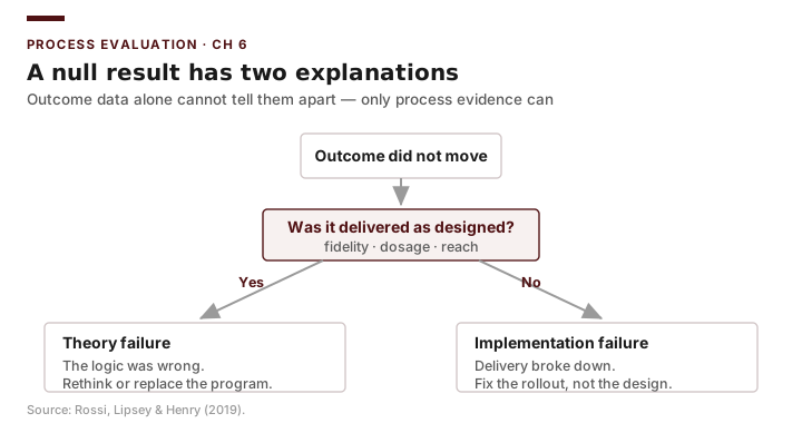
Here is the payoff, and the single most important idea in the chapter. When a program does not produce the outcomes it hoped for, there are two fundamentally different explanations, and telling them apart is impossible without process data (Rossi, Lipsey & Henry 2019).
Theory failure means the program was delivered as designed — good fidelity, adequate dosage, reasonable coverage — and still did not move the outcome. The activities happened; the assumed causal chain simply does not hold in the world. Here the logic model itself is wrong, and the right response is to rethink or abandon the program’s theory of change.
Implementation failure means the program’s theory might be perfectly sound, but the outcome did not move because the program was never really delivered — locations never opened, doses fell short, the eligible went unserved. Here the idea was never actually tested, and abandoning it would be a mistake; the fix is in delivery, not design.
A null impact finding is identical on the outcome side under both explanations, which is why you cannot interpret one without process evidence. Run the five cases through this lens:
- Case B (vote centers). A flat turnout result is theory failure if vote centers were opened and publicized and voters still did not respond; it is implementation failure if, as the monitoring table above illustrates, locations went unopened and publicity was never delivered.
- Case C (NSW). A weak earnings effect is theory failure if the full supported-work dose was delivered and earnings still did not rise; it is implementation failure if enrollees received only a fraction of the intended months of subsidized work.
- Case D (MTO). A muted neighborhood effect is theory failure if families actually moved to low-poverty tracts and their circumstances still did not change; it is implementation failure to the extent that partial take-up meant many families never moved at all.
- Case A (EDC sales tax). A disappointing jobs result is theory failure if incentives were genuinely deployed to recruit firms and firms still did not come; it is implementation failure if the tax revenue was disbursed without any real recruitment activity behind it.
- Case E (Perry Preschool). A weak graduation effect would be theory failure if children attended the full daily preschool and weekly home-visit dose and still did not do better; it would be implementation failure if attendance was spotty or home visits went undelivered. For a small grant-funded nonprofit this is not academic: the funder’s report must document dosage and fidelity precisely so that a disappointing outcome can be read correctly — and so a good outcome can be defended as the program’s own.
In every row, the outcome number cannot distinguish the two diagnoses. Only evidence about fidelity, dosage, reach, and coverage can.
Briefing: A null impact has two faces — the theory was wrong, or the program was never delivered. They demand opposite responses (drop the idea vs. fix delivery), and outcome data alone cannot tell them apart. Never interpret a null without process evidence.
Returning to the Case: The commissioners’ question — “did vote centers not work?” — was unanswerable at the start of the chapter and is answerable now, but only with process evidence in hand. If the monitoring record shows vote centers opened on schedule, staffed, and publicized, then a flat turnout result points toward theory failure: for this county, vote-anywhere polling did not move turnout, consistent with the small, non-significant metro/non-metro gap Chapter 5 already found. If instead the record shows unopened locations and near-absent publicity, the honest report is that the program was never really delivered, the idea remains untested, and the recommendation is to fix the rollout before judging the concept. Same turnout number, opposite recommendations — and process evaluation is the only thing that decides between them.
Common Pitfalls
- Interpreting a null impact without process data. The cardinal error of the chapter: reading “no effect” as “the idea failed” when the program may never have been delivered.
- Counting outputs without a plan to compare against. “9 vote centers opened” is meaningless until set beside the number planned; report actuals against targets, not alone.
- Treating treatment as a switch. Recording who “received the program” as yes/no while ignoring dosage, which is often the variable that explains a weak effect.
- Confusing reach with coverage. A large participant count can still be a small share of the eligible population; a program can look busy and cover almost no one.
- Assuming fidelity. Presuming a program in the field matches the program on paper; drift is the rule, not the exception, and must be measured.
- Reporting process instead of impact — or impact instead of process. They answer different questions. A delivery audit is not evidence of effect, and an effect estimate is not evidence of delivery. Decision-makers usually need both.
Practice and Application
-
Logic model as checklist. Take a logic model you built in Chapter 2 for any running case and convert it into a delivery checklist: for each activity and output box, write the monitoring indicator and the data source that would show it actually happened.
-
Fidelity vs. dosage. For NSW (Case C), write one-sentence definitions of a fidelity question and a dosage question, and explain how a program could score high on one and low on the other.
-
Monitoring table (Excel). Build a four-row planned-vs-actual monitoring table for one case, with a
=Actual/Planneddelivery-ratio column formatted as a percentage. Write two sentences interpreting the pattern of ratios, using clearly labeled illustrative values. -
Coverage rate (Excel). For any case with an eligible population and a served count, compute a coverage rate with
=served/eligible. Explain how partial coverage caps the program’s possible population-level effect, using MTO’s partial take-up (Case D) as the reference example. -
Theory vs. implementation failure. Choose a running case, imagine it produced a null impact finding, and describe the specific process evidence you would gather to decide whether the null reflects theory failure or implementation failure. State what recommendation each diagnosis would imply.
-
Grant report on a shoestring (Case E). You direct a small nonprofit running a Perry-style preschool on a foundation grant, with no evaluation staff. Design a one-page quarterly process report the funder would accept: choose three monitoring indicators (e.g., average days attended, home visits completed, share of enrolled children still active), give each a planned and an actual value in an Excel table with a delivery-ratio column, and write the two-sentence narrative you would send. Explain why reporting delivery honestly — even when a ratio is below plan — protects the program more than a polished outcomes-only summary.
Transition to Chapter 7
Process evaluation establishes whether the program was delivered; the rest of the course returns to whether it worked, now on firmer ground. But the comparisons of Chapter 5 have a limit we have not yet solved: when treatment and comparison groups differ on income, education, and population all at once, a simple mean comparison confounds the program with everything else that distinguishes the groups — and knowing the program was faithfully delivered does not undo that confounding. Chapter 7 introduces regression, which lets us compare groups while holding other characteristics constant, isolating one factor’s contribution from the tangle of others and setting up the quasi-experimental designs that follow.