Chapter 11: Cost-Benefit and Cost-Effectiveness Analysis
Epigraphs
“Cost-benefit analysis is a method of assessing the desirability of projects when it is important to take a long view and a wide view.” — Anthony Boardman, David Greenberg, Aidan Vining, and David Weimer, Cost-Benefit Analysis: Concepts and Practice
Opening Case: Was Job Training Worth the Cost?
In Chapter 10 you met the National Supported Work (NSW) demonstration — a randomized job-training program for disadvantaged workers whose experimental evaluation found that participants earned about $1,794 more in 1978 than their randomized controls (treated mean $6,349 vs. control mean $4,555). Randomization settled the causal question: the program worked, raising earnings.
But a workforce agency cannot stop there. Subsidized work placements, supervision, stipends, and administration all cost real money, and that money could instead fund childcare subsidies, transit passes, or wage subsidies elsewhere. The agency’s board wants to know whether the dollars spent on NSW bought more in earnings and reduced dependence than they cost — and whether the answer holds once you account for the fact that costs are paid up front while the earnings gains accrue over several years.
You are asked to prepare a cost-benefit analysis. Immediately you face two challenges. First, some benefits are easy to monetize (the measured earnings gain, reduced welfare payments) while others are not (a participant’s restored sense of agency, effects on their children). Second, the costs land now but the earnings benefits unfold over years — and a dollar several years from now is not worth a dollar today.
Guiding Questions
- Which costs and benefits belong in the analysis, and how do we attach dollar values to them honestly?
- Why must we discount future dollars, and how do Net Present Value and the benefit-cost ratio summarize a program’s worth?
- When benefits resist monetization — as in MTO’s neighborhood effects — how does cost-effectiveness analysis still let us compare programs?
Why This Chapter Matters
Public budgets are zero-sum in the short run: a dollar spent on job training is a dollar not spent on something else. Cost-benefit analysis (CBA) is the discipline of making that trade-off explicit and defensible. It forces an evaluator to inventory all consequences of a program, value them in common units, and confront the awkward fact that timing matters. Done well, CBA is among the most persuasive products an evaluator can hand a board or council. Done carelessly — with cherry-picked benefits or a self-serving discount rate — it is among the easiest to manipulate. This chapter teaches both the mechanics and the honesty that must accompany them.
Identifying and Valuing Costs and Benefits
The first task is an inventory. List every consequence of the program for every party with standing (whose welfare counts — usually the city’s residents, sometimes a broader public).
Costs include the obvious direct outlays (wages for subsidized placements, supervisor salaries, training materials, administration) and the easily forgotten ones: the opportunity cost of resources already owned, and participant time spent in the program rather than in other work. A common error is to count only what shows up on an invoice.
Benefits are the program’s valued effects. Some are market benefits with observable prices — the measured earnings gain participants take home is the central NSW benefit. Others are non-market benefits requiring valuation techniques: willingness-to-pay surveys, or transferring values estimated elsewhere (benefit transfer).
Briefing: Count opportunity costs, not just cash outlays — and count a benefit once. Double-counting (e.g., adding both higher earnings and the higher consumption those earnings finance, when one is simply the other) inflates the case.
Avoid counting transfers — pure redistributions like a welfare check that takes a dollar from taxpayers and hands it to a participant — as net social benefits. From society’s whole-community perspective, a transfer nets to zero; only real changes in resources (like the increase in output a newly employed worker produces) count. A reduction in welfare payments is a benefit to taxpayers but a loss to the recipient; whether you net it out depends on whose standing you adopt, and you should state that choice explicitly.
The Time Value of Money: Discounting and NPV
A benefit received in year 10 is worth less than the same benefit today, because today’s dollar could be invested and grow. To compare costs and benefits arriving in different years, we discount each future amount back to its present value using a discount rate \(r\). The present value of an amount \(B_t\) received in year \(t\) is:
\[PV = \frac{B_t}{(1+r)^t}\]The Net Present Value of a program with net benefits \(NB_t = B_t - C_t\) in each year \(t\) from \(0\) to \(T\) is:
\[NPV = \sum_{t=0}^{T} \frac{B_t - C_t}{(1+r)^t}\]Briefing: The decision rule is simple — undertake the program if \(NPV > 0\), and when ranking competing programs under a fixed budget, prefer higher NPV.
A related summary is the benefit-cost ratio (BCR), the present value of benefits divided by the present value of costs:
\[BCR = \frac{\sum_{t=0}^{T} B_t / (1+r)^t}{\sum_{t=0}^{T} C_t / (1+r)^t}\]A program is worthwhile when \(BCR > 1\). NPV tells you the magnitude of net value; BCR tells you the value per dollar spent. They can disagree when ranking: a large program may have a higher NPV but a lower BCR than a small, efficient one. For a fixed budget, BCR helps you squeeze the most value per dollar; for an absolute go/no-go decision, NPV is the cleaner guide.
The discount rate \(r\) is the most contested input. A higher rate punishes distant benefits more harshly — bad news for programs like job training or MTO whose earnings payoffs accrue years into the future. There is no single “correct” rate, which is precisely why we test several (below).
Cost-Effectiveness Analysis When Benefits Resist Dollars
Sometimes the central benefit cannot be credibly monetized — and forcing a dollar figure onto “a child raised in a safer neighborhood” or “a life saved” can do more to discredit an analysis than to advance it. Cost-effectiveness analysis (CEA) sidesteps monetization. It expresses cost per unit of a natural outcome:
\[CER = \frac{\text{Present value of costs}}{\text{Units of effect}}\]MTO is a natural CEA candidate. Its most striking results — Chetty, Hendren, and Katz (2016) found that children who moved young earned about 31% more as adults, attended college at higher rates, and lived in better neighborhoods themselves — are partly monetizable (the earnings gain) and partly not (the broader gains in opportunity and well-being). Rather than force a single dollar figure onto every dimension, an analyst might report a cost-effectiveness ratio such as “program cost per additional child who attends college,” or “cost per dollar of additional adult earnings generated.” CEA cannot tell you whether a program is worth doing in the abstract, but it is powerful for comparing programs that share an outcome: if a competing mobility or schooling intervention achieves the same gain at lower cost per child, CEA makes that visible even though the full benefit was never priced in dollars.
Briefing: Use CEA when the key benefit is real but cannot be honestly monetized — MTO’s neighborhood effects are a prime example; it ranks programs sharing a common outcome, but it cannot declare a single program “worth it” on its own.
Sensitivity Analysis
Every CBA rests on assumptions: the discount rate, the size of the effect, how long benefits persist, the dollar value of each benefit. Sensitivity analysis asks how the conclusion changes when those assumptions change. The simplest form varies one input at a time — recomputing NPV across a range of discount rates. A break-even analysis finds the assumption value at which NPV hits zero (e.g., “the program pays off as long as the discount rate stays below 9%”). Honest sensitivity analysis is what separates a persuasive CBA from a sales pitch.
Briefing: A finding that survives a wide range of reasonable assumptions is credible; one that flips when the discount rate moves a point or two should be reported as fragile.
Perry Preschool: The Field’s Most Famous Cost-Benefit Result (Case E)
No cost-benefit result has moved public policy more than Perry Preschool’s, and it illustrates every idea in this chapter at once. The nonprofit spent about $15,166 per child (constant 2000 dollars, 3% discount rate) on one or two years of preschool. Followed to age 40, the program group did better on outcome after outcome; when the analysts valued those differences in dollars and discounted them back, the estimated return to society was about $244,812 per child — roughly $16 for every $1 invested (Schweinhart et al. 2005). To the public budget alone (taxpayers, setting aside the participant’s private gains) the return was about $12.90 per $1.
Three features make Perry the ideal teaching case for honest CBA:
- Most of the benefit is non-market. About 88% of the public return — roughly $171,473 per child — came not from higher taxes on higher earnings but from reduced crime: fewer arrests, trials, incarcerations, and victim costs. This is the valuation problem of the chapter made concrete. A CBA that counted only earnings would have missed seven-eighths of the program’s value, and pricing the crime savings requires defensible assumptions that a skeptic can inspect — exactly the kind of number to expose to sensitivity analysis.
- The long horizon makes discounting decisive. Perry’s benefits accrue over forty years; its costs are paid in the first two. A higher discount rate punishes those distant benefits hard, so the choice of \(r\) is not a technicality — it moves the headline. This is why the result is always reported with its rate (3%), not as a bare ratio.
- It survives a tougher reanalysis. Heckman and colleagues (2010) re-estimated the return with methods that correct for the study’s small-sample and randomization quirks and attach standard errors — and still found a 7–10% annual social rate of return, roughly $7–$12 per $1. The point estimate fell, but the conclusion — benefits comfortably exceed costs — held. A finding that survives a hostile reanalysis is exactly the “robust to reasonable assumptions” result the sensitivity-analysis section prized.
The lesson for a public manager is not that every preschool returns $16 on the dollar — Perry was a small, intensive, well-run program, and later at-scale programs show smaller effects. It is that a rigorous CBA, built on a credible impact estimate and honest about its discount rate and its non-market valuations, can make the case for a program more persuasively than any outcome table alone.
Briefing: Perry shows CBA at its most powerful and most demanding: the headline ($16 per $1) rests on valuing non-market benefits (mostly avoided crime), on a stated discount rate over a 40-year horizon, and on an effect that survived a skeptical reanalysis. Report all three, or the ratio is a sales pitch.
Worked Example: Was NSW Worth It? A Cost-Benefit Model in Excel
We model one NSW participant over six years. We anchor the analysis on the real, experimentally estimated benefit: participants earned about $1,794 more per year than randomized controls (the +$1,794 effect from Chapter 10). We treat that earnings gain as a benefit stream that persists for the first several years after the program.
The program’s cost is where we must be careful. We will not invent a precise NSW cost figure. Instead, for the arithmetic we adopt an explicitly labeled illustrative assumption: suppose the program cost $8,000 per participant, paid entirely up front in year 0. This is a teaching placeholder, not a reported NSW estimate; in a real report you would replace it with documented program-cost data and cite the source. Everything in the benefit column, by contrast, is the genuine experimental finding.
All figures below are in dollars. We lay out one column per year in Excel.
| Year \(t\) | Costs \(C_t\) | Benefits \(B_t\) | Net \(NB_t\) | PV of net at 5% |
|---|---|---|---|---|
| 0 | 8,000 | 0 | \(-8{,}000\) | −8,000.00 |
| 1 | 0 | 1,794 | 1,794 | 1,708.57 |
| 2 | 0 | 1,794 | 1,794 | 1,627.21 |
| 3 | 0 | 1,794 | 1,794 | 1,549.72 |
| 4 | 0 | 1,794 | 1,794 | 1,475.93 |
| 5 | 0 | 1,794 | 1,794 | 1,405.65 |
| 6 | 0 | 1,794 | 1,794 | 1,338.72 |
| Total | +1,105.79 |
The last column discounts each year’s net benefit by \((1+r)^t\) at \(r = 5\%\) — e.g., year 3 is \(1{,}794 / (1.05)^3 = 1{,}549.72\). Its sum is +$1,106, which is the NPV. This is the number you can confirm by hand, not just take on faith from Excel’s NPV function; the two agree exactly.
Step 1 — Lay out the cash flows. Put years in row 1, costs in row 2, benefits in row 3, and net benefits in row 4 with =B3-B2 dragged across. To reproduce the present-value column above, add a row with =B4/(1+$B$8)^B1 dragged across, and sum it — it returns the same +$1,106.
Step 2 — Compute NPV. Excel’s NPV function discounts a stream beginning one period in the future, so it must not include the year-0 value inside the function — add year 0 separately. With the rate in cell B8 (say 5%), net benefits for years 1–6 in C4:H4, and year 0 in B4:
=B4 + NPV(B8, C4:H4)
At 5% this returns about +$1,106 — positive, so on these (real benefit, illustrative cost) figures the program clears the bar.
Step 3 — Compute the BCR. Discount benefits and costs separately. Present value of benefits: =B3 + NPV(B8, C3:H3); present value of costs: =B2 + NPV(B8, C2:H2); then BCR = PV_benefits / PV_costs. At 5% the BCR is about 1.14 — roughly $1.14 of discounted earnings benefit per $1.00 of cost.
Step 4 — Sensitivity table. Build a one-variable Data Table (Data ▸ What-If Analysis ▸ Data Table) that recomputes NPV as the discount rate runs from 2% to 12%. List the rates down a column, point the table at your NPV formula, and Excel fills in the NPV at each rate in one step.
| Discount rate \(r\) | NPV ($) |
|---|---|
| 2% | 2,049 |
| 5% | 1,106 |
| 8% | 293 |
| 12% | \(-624\) |
At low and moderate discount rates the program is a net positive; at high rates the later earnings benefits are discounted too heavily to cover the up-front cost. The break-even rate lies near 9%.
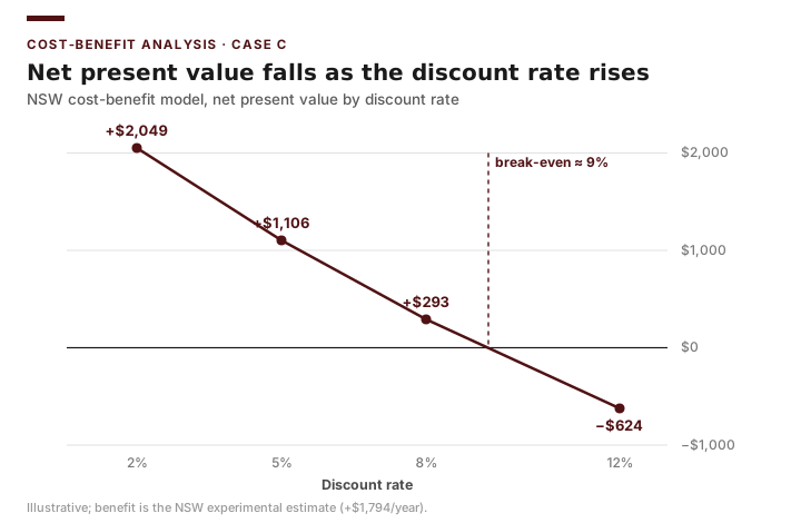
Returning to the Case: You can tell the workforce board that, under these figures, NSW is a net positive investment across the usual range of public discount rates, with a benefit-cost ratio around 1.14 at 5% and a break-even near 9%. Two honesty caveats belong in the same breath. First, the benefit is the real experimental estimate (+$1,794/year), but the $8,000 cost is an illustrative placeholder — your bottom line moves with the true program cost, which is why you report the break-even rate and run the sensitivity table. Second, the published NSW evaluations found that benefits exceeded costs for some target groups — notably long-term welfare recipients — while the case was weaker for others; a credible report would present results by subgroup rather than a single all-in verdict (LaLonde 1986; Dehejia and Wahba 1999). And where a benefit cannot be honestly priced at all — as with MTO’s neighborhood effects — you would switch to the cost-effectiveness framing and let the board compare dollars-per-outcome across competing programs directly.
Common Pitfalls
- Ignoring the time value of money. Summing undiscounted costs and benefits across years overstates programs whose payoffs are far off — exactly the case when an earnings benefit like NSW’s accrues year after year.
- Counting transfers as benefits. A welfare payment moving money from taxpayers to a participant is not a net social gain; be explicit about whose standing you adopt.
- Double-counting. Adding both an intermediate outcome and the final outcome it produces inflates benefits.
- Cherry-picking the discount rate. Choosing the rate that makes your program look best, without disclosing the sensitivity, is advocacy, not analysis.
- Passing off an assumed cost as a measured one. If you must plug in a cost figure you have not documented, label it as an illustrative assumption and test it — never let a placeholder masquerade as a finding.
- Omitting opportunity costs. “Free” donated space or participants’ foregone time still has a value that belongs in the cost column.
- Forcing monetization where it isn’t credible. A made-up dollar value for an intangible (MTO’s neighborhood effects, say) can discredit an otherwise sound analysis; CEA is often the more honest tool.
Practice and Application
- Build the NPV model. Recreate the NSW table in Excel with the real $1,794 annual benefit and the $8,000 illustrative cost, and compute NPV at 5% using
=B4 + NPV(B8, C4:H4). Confirm you get about +$1,106, then change the cost assumption to $10,000 and report how the NPV and your conclusion change. - Benefit-cost ratio. Using the same spreadsheet, compute the BCR at 5% by discounting benefits and costs separately. Confirm it is about 1.14, then interpret in one sentence what a BCR below 1 would mean for the board’s decision.
- Sensitivity Data Table. Build a one-variable Data Table varying the discount rate from 1% to 15%. Identify the break-even rate (near 9% on these figures) and write two sentences on what that implies about how robust the “worth it” conclusion is.
- Cost-effectiveness vs. cost-benefit. Explain in a short paragraph why MTO’s main benefits (a child’s improved life trajectory, safer surroundings) are better handled with cost-effectiveness analysis than with a single monetized cost-benefit figure, and propose one natural-unit ratio you could report for MTO.
- City finance application. Using the Texas city finance panel, propose a small local program (e.g., a downtown facade-improvement grant) whose benefits show up as higher future sales-tax revenue. Sketch a five-year cost-benefit table, clearly label any cost figure you assume rather than measure, name the discount rate you would use, and explain one benefit you would not attempt to monetize.
- Interrogate the $16 (Case E). Perry Preschool reports a societal benefit-cost ratio of about $16 per $1, of which roughly 88% is reduced-crime value. (a) In one paragraph, explain why the choice of discount rate matters so much for a program whose benefits span 40 years but whose costs fall in the first two. (b) The independent Heckman et al. (2010) reanalysis lands at roughly $7–$12 per $1. Explain why the lower estimate arguably makes the case more persuasive to a skeptical council, not less. (c) Name one benefit in the crime-savings figure that you would flag for sensitivity analysis, and say why.
Transition to Chapter 12
You now have a verdict on NSW: a program that works, with a net value that depends visibly on the cost you assume and the discount rate you choose. The final task is the one that determines whether any of this analysis matters — communicating it. A correct NPV buried in a confusing memo persuades no one, and a confident claim that hides its own uncertainty — or quietly passes off an illustrative cost as a measured one — is a breach of professional ethics. Chapter 12 turns to the evaluation report: how to structure findings for busy decision-makers, how to report uncertainty and threats to validity honestly, how to visualize results for non-technical audiences, and how to use new tools — including AI — responsibly without ever surrendering your own judgment.