Chapter 10: Randomized Controlled Trials
Epigraphs
“Randomized experiments are the gold standard for estimating causal effects.” — Donald B. Rubin
“Random assignment is a procedure for creating treatment and control groups that are, on average, identical in every way except the treatment itself.” — Alan S. Gerber and Donald P. Green, Field Experiments (2012)
Opening Case: Moving to Opportunity
In the 1990s, the U.S. Department of Housing and Urban Development launched one of the most ambitious social experiments in American history. The Moving to Opportunity (MTO) demonstration enrolled roughly 4,600 low-income families living in high-poverty public-housing projects in five cities — Baltimore, Boston, Chicago, Los Angeles, and New York. The policy question was old and contested: does growing up in a poor neighborhood itself hold children back, or are the families who live there simply different in ways that would limit their children regardless of address? Decades of observational studies had compared children from poor and non-poor neighborhoods and found large gaps — but skeptics rightly objected that families do not land in neighborhoods at random. The motivated, the employed, the better-connected sort themselves into better places. Any neighborhood “effect” might be nothing more than the selection of who lives where.
MTO broke that deadlock by design. Among families who volunteered, HUD used a lottery to assign each to one of three arms: an experimental group offered a housing voucher that could be used only in a low-poverty neighborhood (plus counseling to help them move), a Section 8 group offered an unrestricted voucher, and a control group offered no new voucher. Because the arm a family landed in was decided by chance, the groups were, on average, alike in motivation, employment history, family structure, and every other trait — measured or not — except the offer they received. For the first time, a difference in their children’s later outcomes could be read as the effect of the offer to move, not the effect of the kind of family that moves.
You will spend this chapter learning why that single design choice — assignment by chance — does what no amount of statistical control can. You will also learn why MTO is the perfect teaching case for what randomization cannot fix on its own: many families offered the experimental voucher never actually moved, so the experiment must carefully separate the effect of being offered the voucher from the effect of using it.
Guiding Questions
- Why does random assignment, and almost nothing else, let us interpret a group difference as a causal effect?
- When many of those offered a program never take it up, what exactly are we estimating — and what should we report?
- What real-world complications — refusal of treatment, dropout, contamination across groups — threaten an experiment even after we randomize?
- Is it ethical, and is it feasible, to assign a public benefit by chance?
Why This Chapter Matters
Every design we have studied so far tries to approximate the comparison a randomized experiment makes directly. Difference-in-differences, matching, and regression with controls all ask, in effect, “what would the treated group have looked like without the program?” and then construct a plausible answer from observational data. A randomized controlled trial (RCT) does not have to construct that answer; it manufactures the counterfactual by design. Understanding the RCT is therefore the conceptual anchor for the entire course. Once you see why randomization works, you can judge how well any weaker design substitutes for it.
Random Assignment and the Logic of Causal Identification
Recall the potential-outcomes framework. For each person \(i\) there are two potential outcomes: \(Y_i(1)\), the outcome if treated, and \(Y_i(0)\), the outcome if not. The individual causal effect is \(Y_i(1) - Y_i(0)\). We can never observe both — this is the fundamental problem of causal inference. We see a person either in the program or out of it, never both.
What we can hope to recover is the average treatment effect (ATE):
\[\text{ATE} = E[Y_i(1)] - E[Y_i(0)]\]The trouble in observational data is that the people we observe as treated are not a fair stand-in for everyone’s \(Y_i(1)\), and the untreated are not a fair stand-in for everyone’s \(Y_i(0)\). Random assignment fixes exactly this. When treatment \(D_i\) is assigned by a coin flip, it is statistically independent of the potential outcomes:
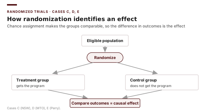
\[E[Y_i(0) \mid D_i = 1] = E[Y_i(0) \mid D_i = 0]\]In words: the control group’s untreated outcome is, in expectation, what the treated group’s outcome would have been without treatment. The control group is a valid counterfactual. The simple difference in group means is then an unbiased estimate of the ATE:
\[\widehat{\text{ATE}} = \bar{Y}_{\text{treatment}} - \bar{Y}_{\text{control}}\]Briefing: Randomization does not make the two groups identical in any single sample — it makes them identical in expectation, balancing both the characteristics you measured and the ones you never thought to measure.
That last clause is the magic. Matching and regression can only balance variables you have data on. Randomization balances everything, including unobserved motivation, family support, and a parent’s drive to find a safer block — the very things that make families who already live in low-poverty neighborhoods a misleading comparison group. In MTO, the lottery is what lets us treat the control families’ later outcomes as a credible picture of how the experimental families’ children would have fared had they not been offered the chance to move.
Designing an RCT
A credible experiment has a few non-negotiable parts:
- A defined population and eligibility rule. In MTO, “families with children living in public housing in selected high-poverty census tracts who volunteered for the demonstration.”
- A treatment and a control condition. Treatment: offer a housing voucher (in MTO’s experimental arm, one usable only in a low-poverty area, plus mobility counseling). Control: no new voucher — the family’s existing situation.
- A randomization mechanism that is genuinely unpredictable and documented — a random-number generator, a sealed-envelope lottery, or a published seed. MTO used a lottery among eligible volunteers.
- Pre-specified outcomes measured the same way for both groups (in MTO, later adult earnings, college attendance, and health, drawn from administrative tax and enrollment records).
Briefing: Decide and write down your outcomes and analysis before you see the data. Choosing the outcome that happens to look best after the fact is a recipe for false findings.
Blinding. In medical trials, neither patient nor doctor knows who got the real drug, which prevents expectations from coloring outcomes. In public programs, blinding the participant to whether they received a voucher is usually impossible — a family knows whether it moved. But you can often blind the people who measure outcomes — the analyst who matches later tax records should not be steered by which arm a family belonged to. That guards against measurement bias even when full blinding is infeasible.
When Reality Intrudes: Attrition, Noncompliance, and Spillovers
Randomization at the moment of assignment is clean. What happens afterward rarely is.
Attrition
Attrition is the loss of subjects from measurement — families who move and cannot be tracked, records that go missing. The danger is not the lost sample size; it is differential attrition. If the families who disappear from one arm differ systematically from those who disappear from the other, the surviving samples are no longer comparable and the estimate is biased. MTO’s long-run follow-ups largely sidestepped this trap by measuring outcomes through administrative tax and college-enrollment records rather than re-interviewing families, so very few subjects were truly lost. Even so, the rule stands: always report attrition rates by arm and check whether the dropouts differ on baseline characteristics.
Noncompliance and ITT vs. Treatment-on-the-Treated
MTO is the textbook illustration of noncompliance. Being offered the experimental voucher did not mean a family used it: take-up was only partial — a large share of families offered the low-poverty voucher never managed to move, whether because they could not find a qualifying unit, faced landlord resistance, or chose to stay near family and familiar schools. Assignment and actual treatment came apart.
You have two honest things to estimate. The intention-to-treat (ITT) effect compares everyone as randomized, regardless of whether they moved. It answers the policy question a HUD administrator cares about: “If we offer this voucher, what happens?” The treatment-on-the-treated (ToT) effect tries to recover the effect on those who actually complied — the families who used the voucher to move. Intuitively, if only a fraction of the offered families moved and the program can only work by changing where a child grows up, the ToT is the ITT scaled up by dividing by the take-up rate — the same total effect concentrated among the families who actually relocated. Two assumptions make this “divide by take-up” shortcut exact: one-sided noncompliance (no control family could obtain the experimental voucher, so no one in the control arm is treated) and the exclusion restriction (being offered the voucher affects earnings only through the move, not in any other way). Both hold well in MTO. Strictly, then, what you recover is the effect on compliers — the families who moved because they were offered the voucher — the local average treatment effect (LATE); here it coincides with the effect on the treated, and it generalizes to families who would have moved anyway only under a further assumption. Because the move was the active ingredient and only some families moved, the effect per complying family is considerably larger than the effect per family offered the voucher.
Briefing: ITT preserves the randomization and is almost always the right headline number for a public decision-maker, because real programs can only offer, not force, participation. The ToT answers a different question — “how much does the program help those who actually use it?” — and in MTO the two differ sharply because take-up was partial.
Spillovers and Contamination
The independence that makes randomization work assumes one person’s treatment does not affect another’s outcome. That can fail. In MTO, the Section 8 arm received unrestricted vouchers, so some control-comparison contrasts had to be read carefully to avoid mixing arms. More generally, if a program changes a shared environment — a school, a labor market, an apartment complex — members of the control group can be indirectly affected, contaminating the comparison and understating (or overstating) the estimated effect. When spillovers are likely, evaluators sometimes randomize at the group level (e.g., by site or by building) rather than the individual level.
Ethics and Feasibility
Is a lottery for a public benefit fair? Often it is more fair than the alternatives, especially when slots are genuinely scarce — a lottery treats every eligible person equally, with no favoritism. MTO’s vouchers were a scarce, sought-after benefit; allocating them by chance among willing volunteers was arguably the fairest mechanism available, and it produced knowledge that has shaped housing policy for a generation. Ethical experiments rest on a few pillars: there should be genuine uncertainty about whether the program helps (equipoise); participants should give informed consent where practical; and the control group should not be denied anything they were already entitled to — MTO’s control families kept their existing housing assistance. A common humane design is the waitlist or phase-in: the control group receives the program later, so the trial only randomizes the order of a benefit everyone eventually gets. Some programs simply cannot be randomized — you cannot randomize which cities get hit by a hurricane — and for those we fall back on the quasi-experimental designs from earlier chapters.
What MTO Found, and Why It Could Be Believed
When Chetty, Hendren, and Katz (2016) linked the MTO families to federal tax records years later, they found that children who moved to a low-poverty neighborhood while young — before about age 13 — went on to earn substantially more as adults. In their mid-twenties these children earned roughly $3,477 more per year (about 31% more) than the control-group children, whose average annual earnings were about $11,270; they were also more likely to attend college and lived in better neighborhoods themselves. Because the move was assigned by lottery, this earnings gap could be attributed to the offer to move into a lower-poverty area rather than to the kind of family that chooses such a neighborhood. (An earlier wave of results — Kling, Liebman, and Katz, 2007 — had found clear gains in adult mental health but limited short-run economic self-sufficiency effects; the long-run earnings payoff for young movers became visible only once the children grew up. This is itself a lesson: when a program’s benefits accrue to children over decades, a short follow-up can mistakenly conclude “no effect.”)
Why Randomization Removes Selection Bias: NSW vs. the Naive Comparison
The clearest demonstration that randomization is doing the heavy lifting comes from the National Supported Work (NSW) demonstration, a job-training experiment that randomly assigned disadvantaged applicants to a subsidized work program or to a control group. Because assignment was random, the honest experimental estimate of the program’s effect on 1978 earnings is simply the difference in arm means: treated participants earned $6,349 on average (n = 185) versus $4,555 for controls (n = 260) — an effect of about +$1,794.
Now suppose you had thrown away the experiment and instead done what observational analysts are forced to do: compare the trained participants to a “comparison group” of non-participants drawn from a national survey. LaLonde (1986) did exactly this and found a negative estimated effect of roughly −$8,498 — the program appeared to destroy earnings. The reason is selection: people who enroll in job training for the disadvantaged start out far poorer than the general population, so a naive comparison loads the dice against the program. Dehejia and Wahba (1999) later showed that careful matching on observed characteristics could partly recover the experimental answer — but only partly, and only because they had the experiment to check against. The lesson is stark: the same program looks like a +$1,794 success under randomization and an −$8,498 disaster under a naive comparison. Randomization is what turns a group difference into a causal effect.
A Small, High-Compliance RCT: Perry Preschool (Case E)
MTO and NSW are large experiments. Perry Preschool (Case E) shows that the same logic governs a tiny one. A nonprofit randomly assigned just 123 children — 58 to preschool, 65 to none — and followed them for decades. Two features make it a clean teaching contrast with MTO. First, compliance was high: nearly all children assigned to the program actually attended, so the offer-versus-received gap that forces MTO’s ITT/ToT distinction barely arises — here the intention-to-treat effect is, for practical purposes, the effect of the program. Second, the outcomes are binary, so the arm comparison is a two-proportion test (Chapter 5) rather than a difference in means: 65% of the program group versus 45% of the comparison group graduated from a regular high school, a 20-percentage-point gap that — despite the tiny sample — reaches significance (\(z \approx 2.3\), \(p \approx 0.02\)), and 36% versus 55% were arrested five or more times.
The small sample is exactly the point. With 123 children the estimates carry wide confidence intervals, and a genuinely small effect would have been undetectable — a real risk that a well-run program can look null purely for want of subjects (the statistical power problem). But Perry’s effects were large enough to clear that bar. The honest report of a small RCT states the effect and its imprecision, and leans on replication — the later Abecedarian and Head Start–era studies — rather than on one small sample, for external validity. Small-N does not mean unrigorous; it means the design must be clean and the uncertainty stated plainly.
Briefing: A randomized experiment with only ~120 subjects is still an experiment: randomization removes selection bias regardless of sample size. What a small sample costs is precision — wide intervals and low power — so a small RCT can credibly detect only large effects, and its generalization rests on replication.
Worked Example: Analyzing a Randomized Experiment in Excel
We will analyze the NSW experiment exactly as you would any RCT: as a difference in means, which is identical to a regression of the outcome on a treatment indicator. Lay out one row per participant with columns treat (1 = job-training arm, 0 = control) and earn78 (1978 earnings in dollars). The treated arm has 185 people, the control arm 260.
Step 1 — Check balance. Before trusting the randomization, confirm the arms look similar on baseline traits. Use AVERAGEIF to compare, say, pre-program (1975) earnings by arm: =AVERAGEIF(treat_range, 1, earn75_range) versus =AVERAGEIF(treat_range, 0, earn75_range). In NSW the arms were close on baseline earnings — the sign of a sound lottery.
Step 2 — Estimate the effect. Compute each arm’s average 1978 earnings with AVERAGEIF on the earn78 column: =AVERAGEIF(treat_range, 1, earn78_range) gives the treated mean, =AVERAGEIF(treat_range, 0, earn78_range) the control mean. The difference is the estimated treatment effect.
Step 3 — Test it. Run the ToolPak’s t-Test: Two-Sample Assuming Unequal Variances (Data ▸ Data Analysis), with the treatment arm’s earn78 values as Variable 1 and the control arm’s as Variable 2. Equivalently — and this scales to adding controls later — run Regression with earn78 as Y and treat as the single X. The coefficient on treat is the difference in means, and its p-value tests the same hypothesis.
| Quantity | Result |
|---|---|
| Control mean earnings \(\bar{Y}_{C}\) (n = 260) | $4,555 |
| Treatment mean earnings \(\bar{Y}_{T}\) (n = 185) | $6,349 |
| Estimated treatment effect | \(+\$1,794\) |
Regression coef. on treat |
\(+\$1,794\) |
| Naive (non-experimental) comparison, for contrast | \(-\$8,498\) |
The positive coefficient says assignment to the job-training program raised 1978 earnings by about $1,794. The final row is the cautionary contrast: had you compared trainees to an ordinary survey sample instead of to randomized controls, you would have estimated a $8,498 loss — a sign-flipping artifact of selection, not a real effect.
Returning to the Case: MTO and NSW make the same point from two directions. Because both used a lottery, the difference in arm means is a credible causal effect — MTO’s young movers earned about 31% more as adults, and NSW’s trainees earned about $1,794 more. And because NSW also has a naive non-experimental benchmark, it shows what you avoid by randomizing: an estimate that comes out −$8,498 and gets the very sign of the effect wrong. When you report MTO, you would lead with the ITT — the effect of being offered the voucher — because HUD can only offer, not compel, a move; you would then note that the effect among families who actually moved (the ToT) is larger, since take-up was only partial; and you would document how outcomes were tracked so readers can judge attrition.
Common Pitfalls
- Reporting the ToT as if it were the program’s overall effect. A policymaker authorizes an offer, not guaranteed participation; lead with the ITT. In MTO, the per-mover effect is real but answers a narrower question than “what does the voucher offer accomplish?”
- Ignoring differential attrition. A clean randomization can still produce a biased estimate if the groups are measured unequally afterward.
- Analyzing only compliers as a self-contained group. Comparing the MTO families who moved to the control families who didn’t throws away the randomization and reintroduces selection bias — the original sin you used the experiment to avoid. (This is exactly the trap NSW’s −$8,498 naive estimate illustrates.)
- Treating a statistically significant difference as a large or important one. Significance and magnitude are different questions; always report the effect size.
- Forgetting that small samples can be imbalanced by chance. Always check baseline balance even after a valid lottery.
- Concluding “no effect” from a follow-up that ends too soon. MTO’s earnings payoff for young movers was invisible in the short run and emerged only once the children reached adulthood.
Practice and Application
- Balance check. Using the Texas county panel, pretend you will randomize 254 counties into a “treatment” and “control” arm with Excel’s
RAND()function and a 0.5 cutoff. After assigning, useAVERAGEIFto compare median household income across your two random arms. Are they close? Repeat the randomization three times and comment on how much the balance varies sample to sample. - ITT vs. ToT reasoning. Suppose only half of the MTO families offered the experimental voucher actually used it to move, and the ITT effect on adult earnings is $1,000 per offered family. Give an intuitive (back-of-envelope) estimate of the ToT effect — the effect per family that moved — and explain in two sentences which number you would put in a HUD executive summary and why.
- Selection bias by hand. Using the NSW numbers in the worked example, state in your own words why the experimental estimate (+$1,794) and the naive comparison (−$8,498) differ so dramatically, and what feature of the people who enroll in job training drives the naive estimate negative.
- Attrition diagnosis. You learn that 15% of the treatment arm and 30% of the control arm could not be located at follow-up. Explain how this pattern could bias the estimated effect, and state the direction of the likely bias.
- Excel regression. Build a small mock dataset with
treat(1/0) and a continuous outcome (e.g., 1978 earnings) whose arm means reproduce the NSW result (treated ≈ $6,349, control ≈ $4,555). Run the ToolPak Regression of the outcome ontreat, confirm the coefficient is about $1,794, and write one sentence interpreting it and its p-value for a non-technical reader. - Small-N RCT (Case E). Perry Preschool randomized 58 children to preschool and 65 to none, with high-school graduation of 65% versus 45%. Compute the two-proportion z-test (Chapter 5) and confirm the gap is significant despite n = 123. Then explain in two or three sentences (a) why the near-full attendance makes the ITT and treatment-on-the-treated effects nearly identical here, unlike MTO, and (b) why you would still cite replication studies rather than Perry alone when arguing the result generalizes.
Transition to Chapter 11
MTO and NSW answered whether the programs work: a move to a lower-poverty neighborhood raised children’s adult earnings, and job training raised participants’ earnings by about $1,794 a year. The next question is harder: is it worth it? A voucher, mobility counseling, and a year of subsidized work all cost money — and the earnings benefits arrive over years while the costs are paid up front. Chapter 11 turns to cost-benefit and cost-effectiveness analysis, where we learn to put costs and benefits on a common footing, account for the time value of money, and decide whether a program that works is a program worth funding.